Step 03
Laying out the plan and getting the data
I address the short-term effects of climate shocks on informality by combining labor data with satellite-derived climate data in a panel regression framework.
I estimate coefficients using a two-way fixed-effect panel regression. The baseline specification is as follows:
where indexes states and denotes the period (annual period from June to July). is the informal employment share, and is the climate shock index: either the yearly drought index or the yearly flood index. I include optimal lags as determined by a BIC analysis (3 lags for the drought index, 2 for the flood index). I control for state- () and time-fixed () effects, and include state-specific linear time trends (to account for state-specific development paths, urbanization, and sectoral shifts). Standard errors are clustered at the state level, and all regressions are weighted by 2020 population.
This recipe (analysis) requires a few ingredients:
- a set of state- and year- specific informality values
- a set of state- and year- specific climate shock indicators (one each for drought and floods)
- population per state, to use as weight and make more populated states more influential on the coefficients (to reflect the actual affected population)
Specific instructions on data retrieval, along with all my code, is decribed in the thesis manuscript (download it at the bottom of the page) and on my Github.
Construction of the informality share
Some Info on the Labor data: Periodic Labor Force Survey of India (PLFS)▶
- Representative national household survey
- Yearly from 2017 to 2024, for each of the 36 states and union territories
- Open access, upon request
More info on survey design: https://www.dataforindia.com/plfs-explainer/
Index construction ▶
My main measure of informality is the share of casual workers among all workers aged 15 to 64. Casual worker status is defined as including individuals who worked in a household enterprise (self-employed) as own account workers or helpers, as casual wage labor in public works, or as casual wage labor in other types of work. This excludes individuals who worked as employers in a household enterprise or as salaried or regular-wage workers. Note that begging and prostitution are excluded from the labor force (as per the PLFS classification).
The status of a casual worker is determined if an individual engaged in casual work as a primary or subsidiary activity (≥ 30 days) over the past 365 days.
I also compute the share of informality for each state for males and females (other genders represent a tiny, if not invisible, fraction of the survey respondents, so they are excluded), and rural and urban areas separately. Additionally, I generate state splits based on the share of agricultural employment and state income [I also tested for geography (north-east, south, ...) but found no significant results, so I dropped it].
Construction of the climate shock indicators
Why satellite data?
Risk = hazard × vulnerability × exposure. I focus on capturing hazard and therefore try to get data as objective and unaffected by human decisions. Damage data reflects part of vulnerability. Satellite data is more objective than station data because it is likely that stations are unevenly distributed, and richer states may have different infrastructure than poorer states, creating a bias.
Note that I do integrate some exposure, since I am weighing events by population living in the area of the event, but I assume that exposure was not chosen, i.e., people could not determine they would be exposed to those threats when they established their livelihoods in those areas.
Drought index ▶
The drought index is based on the SPEI-12 index, which looks at temperature and evapotranspiration over the past 12 months. Values are normalized at the pixel level so that a negative score indicates a negative deviation (drought) compared to the baseline. I filter out the positive values and keep only the negative values, so that my index reflects the intensity of a drought.
My workflow for the index construction from satellite to state-year index is the following
- Download SPEI (12 months) gridded data (0.25° resolution) from Copernicus
- Compute population per district and average SPEI per district
- Aggregate to state level using population weight
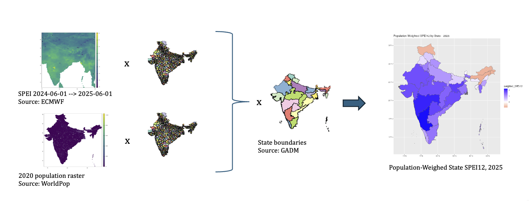
Sources: ECMWF (SPEI), WorldPop (population), GADM (state boundaries).
Flood index ▶
Building the flood index was much less straightforward than the drought index. But it was also a lot more fun and required more investigation. It seems there is no unanimous approach to measuring floods in environmental economics. Floods are complex and can be broken down into three main categories: flash floods, fluvial floods, and coastal floods. Keeping the rationale of focusing on the hazard, and because of my technical expertise, I focus on flash floods (fluvial and coastal floods reflect, to some extent, human decisions in establishing in that area, and their damage will also depend on land use choices and infrastructure - many more variables than just precipitation intensity).
What's a flash flood? Essentially, very intense precipitation over the course of a few hours. Those can be very destructive (I go into more details in Results, as I explain the observed motions).
So how do I go about measuring them? I capture the year's worst hit by flash floods by counting the number of extreme events that occurred in that year in a given state, weighing the events within the state by how many people live in the affected area.
But what counts as an extreme event? For each district, I ask, "If I wait 10 years, what’s the worst event I can reasonably expect? How many times was this value exceeded?" This is known as "return period value exceedance" (common in insurance). You can find the details of my process in the thesis itself; here's the overview. Ah yes, also, because research suggests that when the soil is drier, it is much harder for water to penetrate, so that very dry soil amplifies the intensity of flash floods [think of the animation on the website's welcome page]. Essentially, I start by looking at precipitation, calculate the extreme threshold, and count how many times it is surpassed, multiplying it by a multiplier so that if the soil was drier than usual at that location on that day, the event counts as stronger.
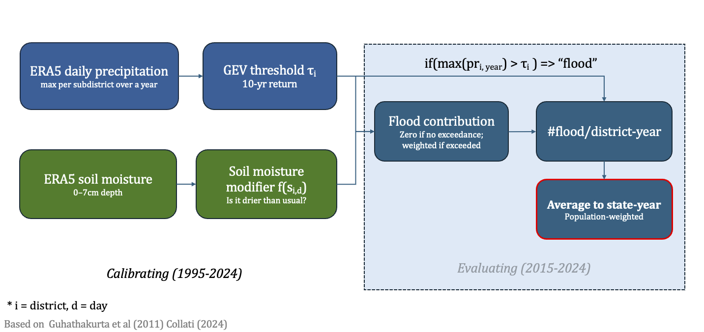 12AB34
Sources: ECMWF (ERA5-LAND, via Google Earth Engine), WorldPop (population), GADM (state boundaries).
State by state
Pick an indicator to see how it varies across the 35 states and union territories in the sample (Lakshadweep excluded). Hover a state for its value.
State-level summary statistics. SPEI, flood and extreme precipitation indices are period means; agricultural share of employment and baseline informality (casual labour share) are reported where available.